

1.2. Standard Inputs#
All problem types require standard input data: cross-sectional data, material locations, spatial discretization, angular quadrature, and source/boundary conditions. These are passed to solver functions as typed dataclass objects — see DataTypes Reference for a complete reference and worked examples.
1.2.1. Cross-Sectional Data#
The neutron cross-sectional data required are:
Total cross section: \(\sigma^{\mathrm{t}}\) — shape \((M \times G)\)
Scattering matrix: \(\sigma^{\mathrm{s}}\) — shape \((M \times G \times G)\)
Fission matrix: \(\chi \, \nu \, \sigma^{\mathrm{f}}\) — shape \((M \times G \times G)\)
where \(M\) is the number of materials and \(G\) is the number of energy groups.
Energy groups are ordered from fastest to slowest (group 0 is the highest energy), and the
scattering and fission matrices are indexed [material, group out, group in].
For anisotropic scattering, the scattering matrix has the
Legendre moments \(\ell = 0, \ldots, L\) on a last axis, shape
\((M \times G \times G \times (L + 1))\), indexed
[material, group out, group in, moment]. The moments do not include the
\((2\ell + 1)\) factor (see anisotropic scattering).
All one- and two-dimensional solvers, and the three-dimensional fixed source solver,
select anisotropic scattering from the shape of the scattering matrix. Two- and
three-dimensional problems use the same Legendre moments, which are expanded into
spherical harmonics internally: the \((L + 1)(L + 2) / 2\) harmonics even in
\(\mu_z\) in 2D, and all \((L + 1)^2\) harmonics in 3D.
# One group P2 scattering
scatter = np.array([[[[0.733333, 0.2, 0.075]]]])
1.2.1.1. Energy Grids#
The NJOY, Serpent, CASMO, SCALE, and other standard group structures are included with ANTS. All energy bounds are in eV and descending order.
edges_g = ants.get_structure("casmo_70")
ants.list_structures("njoy")

# Bounds and coarsening indices (here 70 fine groups to 10 coarse groups)
edges_g, edges_gidx_fine, edges_gidx_coarse = ants.energy_grid("casmo_70", 70, 10)
- ants.get_structure(name)[source]#
Return a standard energy group structure by name.
- Parameters:
name (str) – Structure identifier (case-insensitive), e.g.
"casmo_70","scale_252","lanl_618","njoy_ign22".- Returns:
edges_g – Energy group bounds in eV, descending (group 0 is the fastest).
- Return type:
ndarray, shape (groups + 1,)
- Raises:
KeyError – If
nameis not a known structure.
- ants.energy_grid(grid, groups_fine, groups_coarse=None, optimize=True)[source]#
Calculate energy grid bounds and index for coarsening
All energy grids are returned in eV and descending order (group 0 is the fastest group). Named structures (e.g.
"casmo_70","lanl_618") come fromants.list_structures(). The integer grids 361 and 618 are the public SHEM-361 and LANL-618 structures, while 87 requires the local (unreleased)ants/sources/data. Any othergridvalue returns unitless edges (0, 1, …, groups_fine).- Parameters:
grid (str or int) – energy structure name, or 87, 361, 618
groups_fine (int) – Number of fine energy groups for problem
groups_coarse (int) – Number of coarse energy groups for problem
optimize (bool) – Whether to use predetermined group edges (Default True)
- Returns:
energy group bounds (eV, descending) edges_gidx_fine (int [groups + 1]): Location of fine grid index for problem edges_gidx_coarse (int [groups + 1]): Location of coarse grid index for problem
- Return type:
edges_g (float [grid + 1])
1.2.1.2. Cross Section Libraries#
Macroscopic cross sections are built from number densities (atoms/barn-cm) and a
HDF5 multigroup library (requires pip install ants-sn[library]). Compositions
can be copied directly from MCNP or PARTISN input decks, and the common materials
(enriched uranium, uranium hydride, enriched plutonium, …) are available by name.
library = ants.Library("endf_xmas172.h5")

# MCNP material card or PARTISN material block
fuel = ants.create_material("m1 94239.80c 3.7047E-02 31069.80c 8.3603E-04", library)

# Named materials and compositions
mat_data = ants.materials(172, ["uranium-%20%", "stainless-steel-440",
                                {"H-1": 0.0668, "O-16": 0.0334}], library=library)

# P3 anisotropic scattering, shape (materials, groups, groups, 4)
fuel = ants.create_material("m1 94239.80c 3.7047E-02", library, legendre=3)
- ants.materials(groups, materials, key=False, datatype=True, library=None, temperature=None)[source]#
Create cross sections for one or more materials.
- Parameters:
groups (int) – Number of energy groups.
materials (list[str or dict]) – Named materials (e.g.
"uranium-%20%") or compositions (seeparse_composition). Compositions require alibrary.key (bool, optional) – If
True, also return the material index mapping.datatype (bool, optional) – If
True, return aMaterialDataobject.library (str or Library, optional) – HDF5 cross section library (or path to it). If
None, the localants/sources/materialsdata are used.temperature (float, optional) – Library temperature (K); the nearest available is used.
- Returns:
Either a
MaterialDatainstance or raw arrays, with the material key map appended ifkeyisTrue.- Return type:
MaterialData or tuple
- ants.create_material(composition, library, temperature=None, legendre=0)[source]#
Create cross sections for one material from number densities.
- Parameters:
composition (dict, list, or str) – Nuclides and number densities (atoms/barn-cm), in any form accepted by
parse_composition(e.g. text copied from an MCNP material card or PARTISN material block).library (str or Library) – HDF5 cross section library (or path to it).
temperature (float, optional) – Temperature (K); the nearest library temperature is used.
legendre (int, optional) – Legendre order of the scattering (0 for isotropic P0 scattering).
- Returns:
Cross sections of shape
(1, groups[, groups]).- Return type:
MaterialData
- ants.parse_composition(composition)[source]#
Convert a composition to normalized nuclide number densities.
- Parameters:
composition (dict, list, or str) – Nuclides and number densities (atoms/barn-cm) as a dictionary, a list of
(nuclide, density)pairs, or text copied from an input deck, e.g. the body of an MCNP material card"94239.80c 3.7047E-02 31069.80c 8.3603E-04"or a PARTISN block'"94239.700nm" 0.037047 "31069.700nm" 0.00083603'. Card names (m1) andkeyword=valueentries are ignored. Natural elements are expanded into isotopes.- Returns:
Nuclide names and number densities (atoms/barn-cm).
- Return type:
dict[str, float]
- class ants.library.Library(path)[source]#
An HDF5 multigroup cross section library.
- Parameters:
path (str or os.PathLike) – Path to the HDF5 library file (layout in the module docstring).
- path#
Library file path.
- Type:
str
- groups#
Number of energy groups.
- Type:
int
- edges_g#
Energy group bounds in eV, descending.
- Type:
ndarray, shape (groups + 1,)
- library_type#
"microscopic"or"macroscopic".- Type:
str
- macroscopic(composition, temperature=None, legendre=0)[source]#
Build macroscopic cross sections from number densities.
- Parameters:
composition (dict[str, float]) – Nuclide names (library keys) and number densities (atoms/barn-cm).
temperature (float, optional) – Temperature (K); the nearest available temperature is used.
legendre (int, optional) – Legendre order L of the scattering (0 for P0 only).
- Returns:
xs_total (ndarray, shape (groups,))
xs_scatter (ndarray, shape (groups, groups[, L + 1]))
xs_fission (ndarray, shape (groups, groups)) – Macroscopic cross sections (1/cm), indexed
[out, in].
- materials(compositions, temperature=None, groups=None, legendre=0)[source]#
Build
MaterialDatafor several materials.- Parameters:
compositions (list[dict[str, float]]) – Nuclide names and number densities (atoms/barn-cm) for each material.
temperature (float, optional) – Temperature (K); the nearest available temperature is used.
groups (int, optional) – Collapse to fewer energy groups. The collapse uses energy bin width weighting, not flux weighting; for a different energy structure build a library at that structure instead.
legendre (int, optional) – Legendre order L of the scattering. 0 (default) gives P0 scattering, shape
(materials, groups, groups); L > 0 gives shape(materials, groups, groups, L + 1).
- Returns:
Cross sections of shape
(materials, groups[, groups])with the neutron velocity of each group.- Return type:
MaterialData
- microscopic(nuclide, temperature=None, legendre=0)[source]#
Load the microscopic cross sections of a single nuclide.
- Parameters:
nuclide (str) – Nuclide name in the library, e.g.
"U-235".temperature (float, optional) – Temperature (K); the nearest available temperature is used.
legendre (int, optional) – Legendre order L of the scattering. 0 (default) returns the P0 scatter matrix; L > 0 returns moments 0 to L on a last axis.
- Returns:
total (ndarray, shape (groups,)) – Total cross section (barns).
scatter (ndarray, shape (groups, groups) or (groups, groups, L + 1)) – Scatter cross section, indexed
[out, in]or[out, in, l](barns).fission (ndarray, shape (groups, groups)) – Fission matrix chi * nu * sigma_f, indexed
[out, in](barns).
1.2.1.3. ICSBEP Benchmarks#
The geometry, material layout, and number densities of ICSBEP criticality benchmarks
(ants.list_benchmarks()) are included, so the same benchmark can be run with any
number of cells, angles, and energy groups. The data are from the International
Handbook of Evaluated Criticality Safety Benchmark Experiments, NEA/NSC/DOC(95)03
(OECD-NEA, September 2015); the full evaluations are available from the NEA, and
publications using these benchmarks should cite the Handbook.
materials, geometry, quadrature, solver = ants.build_problem(
    "PU-MET-FAST-001", library, cells=200, angles=8
)
results = ants.run_suite(ants.list_benchmarks("MET-FAST"), library,
                         cells=[100, 400], angles=[4, 8, 16])
- ants.build_problem(benchmark, library, cells, angles, groups=None, temperature=None, legendre=0)[source]#
Create the ANTS k-eigenvalue problem for an ICSBEP benchmark.
- Parameters:
benchmark (str or Benchmark) – Benchmark name or specification.
library (str or Library) – HDF5 cross section library (or path to it).
cells (int or list[int]) – Total number of spatial cells, divided between the regions in proportion to their thickness, or the number of cells per region. Region boundaries always fall on cell edges.
angles (int) – Number of discrete ordinates.
groups (int, optional) – Collapse the library to fewer energy groups (energy bin width weighting). Defaults to the library groups.
temperature (float, optional) – Library temperature (K); defaults to the benchmark temperature.
legendre (int, optional) – Legendre order of the scattering (0 for isotropic P0 scattering).
- Returns:
materials (MaterialData)
geometry (GeometryData)
quadrature (QuadratureData)
solver (SolverData)
- ants.run_suite(names, library, cells=(100,), angles=(8,), groups=(None,), temperature=None, legendre=0)[source]#
Run k-eigenvalue calculations over a suite of ICSBEP benchmarks.
- Parameters:
names (list[str]) – Benchmark names (see
list_benchmarks).library (str or Library) – HDF5 cross section library (or path to it).
cells (list[int]) – Values to run for every benchmark (all combinations).
Noneingroupsuses the library groups.angles (list[int]) – Values to run for every benchmark (all combinations).
Noneingroupsuses the library groups.groups (list[int]) – Values to run for every benchmark (all combinations).
Noneingroupsuses the library groups.temperature (float, optional) – Library temperature (K); defaults to each benchmark temperature.
legendre (int, optional) – Legendre order of the scattering (0 for isotropic P0 scattering).
- Returns:
One row per run with keys
name,groups,angles,cells,legendre,keff,reference,uncertainty, anddiff_pcm(calculated minus benchmark k, in pcm).- Return type:
list[dict]
1.2.1.4. Kobayashi Benchmarks#
The three-dimensional Kobayashi benchmarks are one-group source problems with a void cube (Problem 1), a straight void duct (Problem 2), or a dog leg void duct (Problem 3) in a shield. Case i is a pure absorber with exact reference fluxes, and case ii has 50% scattering with Monte Carlo reference fluxes. The problems and reference values are from K. Kobayashi, N. Sugimura, and Y. Nagaya, 3-D Radiation Transport Benchmark Problems and Results for Simple Geometries with Void Regions, NEA/NSC/DOC(2000)4 (OECD-NEA, 2000).
from ants.benchmarks import kobayashi
from ants.fixed3d import fixed_source

inputs = kobayashi.build_problem(3, scattering=True, cell_width=2.0, angles=8)
flux = fixed_source(*inputs)
points, reference, uncertainty = kobayashi.reference("3C", scattering=True)
approx = kobayashi.flux_at(flux[..., 0], points, inputs[2])
- ants.benchmarks.kobayashi.build_problem(problem, scattering=False, cell_width=2.0, angles=8, space_disc=SpatialDiscretization.STEP_CHARACTERISTIC, solver=None)[source]#
Create the ANTS inputs for a Kobayashi benchmark problem.
- Parameters:
problem (int) – Problem number (1, 2, or 3).
scattering (bool, optional) – If True, case ii (50% scattering), otherwise case i (pure absorber).
cell_width (float, optional) – Width of the cubic spatial cells (cm). Every 10 cm must hold an odd number of cells so the reference points are at cell centers.
angles (int, optional) – Number of angles in each direction for
ants.angular_xyz.space_disc (SpatialDiscretization, optional) – Spatial discretization. The default is step characteristic, since diamond difference gives negative fluxes in the shield.
solver (SolverData, optional) – Solver options. The default is
SolverData().
- Returns:
materials (MaterialData) – Source (0), void (1), and shield (2) cross sections.
sources (SourceData) – Unit source in the source region and vacuum boundaries.
geometry (GeometryData) – Medium map and cell widths.
quadrature (QuadratureData) – Angles ordered for the reflecting faces.
solver (SolverData) – Solver options.
- ants.benchmarks.kobayashi.reference(case, scattering=False)[source]#
Reference total flux of a Kobayashi benchmark case.
- Parameters:
case (str) – Set of points,
"1A","1B","1C","2A","2B","3A","3B", or"3C". The first character is the problem.scattering (bool, optional) – If True, case ii (50% scattering), otherwise case i (pure absorber).
- Returns:
points (ndarray, shape (points, 3)) – (x, y, z) location of each point (cm).
flux (ndarray, shape (points,)) – Reference total flux (cm^-2 s^-1).
uncertainty (ndarray, shape (points,)) – Fractional standard deviation of the Monte Carlo flux for case ii, and zeros for the exact case i values.
- ants.benchmarks.kobayashi.flux_at(flux, points, geometry)[source]#
Scalar flux of the cells holding each point.
- Parameters:
flux (ndarray, shape (cells_x, cells_y, cells_z) or (..., groups)) – Scalar flux from
ants.fixed3d.fixed_source.points (ndarray, shape (points, 3)) – (x, y, z) location of each point (cm).
geometry (GeometryData) – Geometry used for the flux.
- Returns:
Flux of the cell holding each point. A point on an edge between two cells takes the cell above it, except on the upper boundary.
- Return type:
ndarray, shape (points,) or (points, groups)
1.2.2. Material Locations#
Material locations are specified using a medium_map array that identifies which
material occupies each spatial cell:
1D problems:
medium_mapis shape \((I,)\) with integer values in [0, M-1]2D problems:
medium_mapis shape \((I \times J,)\) with integer values in [0, M-1]3D problems:
medium_mapis shape \((I \times J \times K,)\) with integer values in [0, M-1]
For structured spatial layouts, use these utility functions:
- ants.spatial1d(layers, edges_x)[source]#
Create a one-dimensional material medium map.
- Parameters:
layers (list of [int, str, str]) – Each entry is
[index, material_name, regions]whereregionsis a comma-separated list of"start - stop"pairs in cm. Example:[0, "plutonium", "0 - 2, 3 - 4"].edges_x (ndarray, shape (cells_x + 1,)) – Spatial cell edge locations in cm.
- Returns:
medium_map – Material index for each spatial cell.
- Return type:
ndarray of int32, shape (cells_x,)
- ants.spatial2d(medium_map, value, coordinates, edges_x, edges_y)[source]#
Populating 2D medium_map with rectangular geometries
- Parameters:
medium_map – 2D medium_map array of size (I x J) to input value, must be of type np.int32
value (int) – Integer to be populating the medium_map. It will correspond to the ordering of the cross section materials
coordinates – list of locations, where each location is composed of the starting index tuple, the length in the x direction and the length in the y direction, with all values being in centimeters. I.E. location = [(x1, y1), dx, dy].
edges_x – Array of length I + 1 with the location of the cell edges in the x direction
edges_y – Array of length J + 1 with the location of the cell edges in the y direction
- Returns:
medium_map populated with value at specific coordinates
- ants.spatial3d(medium_map, value, coordinates, edges_x, edges_y, edges_z)[source]#
Populate a 3D medium_map with rectangular boxes.
- Parameters:
medium_map (ndarray of int32, shape (cells_x, cells_y, cells_z)) – Medium map to fill.
value (int) – Material index to place in each box.
coordinates (list of [(float, float, float), float, float, float]) – Each box is
[(x1, y1, z1), dx, dy, dz], the starting corner and the lengths in x, y, and z in cm. Every face must lie on a cell edge.edges_x (ndarray, shape (cells_x + 1,)) – Spatial cell edge locations in x in cm.
edges_y (ndarray, shape (cells_y + 1,)) – Spatial cell edge locations in y in cm.
edges_z (ndarray, shape (cells_z + 1,)) – Spatial cell edge locations in z in cm.
- Returns:
medium_map – Medium map with
valueplaced in each box.- Return type:
ndarray of int32, shape (cells_x, cells_y, cells_z)
Three-dimensional maps that are axial stacks of two-dimensional layouts (an assembly with top and bottom reflectors, for example) can be built from the 2D maps directly:
- ants.extrude3d(layers, edges_z)[source]#
Create a 3D medium map by stacking 2D medium maps along z.
- Parameters:
layers (list of [ndarray, str]) – Each entry is
[medium_map, regions]wheremedium_mapis a 2D map of shape(cells_x, cells_y)andregionsis a comma-separated list of"start - stop"pairs along z in cm. Example:[fuel_map, "0 - 21.42"].edges_z (ndarray, shape (cells_z + 1,)) – Spatial cell edge locations in z in cm.
- Returns:
medium_map – Material index for each spatial cell.
- Return type:
ndarray of int32, shape (cells_x, cells_y, cells_z)
1.2.3. Spatial Data#
Spatial discretization requires cell widths in each direction:
1D problems:
delta_x— array of cell widths, shape \((I,)\)2D problems:
delta_xanddelta_y— shapes \((I,)\) and \((J,)\) respectively3D problems:
delta_x,delta_y, anddelta_z— shapes \((I,)\), \((J,)\), and \((K,)\) respectively
1.2.4. Angular Data#
Angular quadrature data (discrete directions and weights) is generated automatically
and returned as a QuadratureData object. With reflecting boundaries, pass the
same bc_x, bc_y, and bc_z to the quadrature as to GeometryData. The
angular flux, the flux at cell edges, and artificial scattering sweep each ordinate
once, so the reflection of an ordinate has to be swept before it. fixed2d and
fixed3d raise an error if the quadrature is not ordered for the boundaries.
- ants.angular_x(angles, bc_x=[0, 0], datatype=True)[source]#
Compute 1D Gauss-Legendre quadrature angles and weights.
- Parameters:
angles (int) – Number of angles (int) or problem info dict with keys
"angles"and"bc_x"(list of two ints, 1 = reflected boundary).- Returns:
angle_x (ndarray, shape (angles,)) – Quadrature direction cosines, ordered for boundary conditions.
angle_w (ndarray, shape (angles,)) – Normalized quadrature weights summing to 1.
- ants.angular_xy(angles, bc_x=[0, 0], bc_y=[0, 0], datatype=True, method='product')[source]#
Compute 2D quadrature angles and weights for slab geometry.
Builds a quadrature set, keeps only the directions with positive polar cosine (upper hemisphere), and reorders them to satisfy reflective boundary conditions.
- Parameters:
angles (int) – Number of angles per dimension. For
method="ldfe"onlyanglesin {4, 8, 16} are available (LDFE-SA levels 1-3).bc_x (list of two ints, optional) – Boundary conditions in the x-direction (default is [0, 0]).
bc_y (list of two ints, optional) – Boundary conditions in the y-direction (default is [0, 0]).
datatype (bool, optional) – If True, return a QuadratureData object. If False, return raw arrays.
method (str, optional) – Quadrature family: “product” (Legendre x Chebyshev, default) or “ldfe” (LDFE-SA from Jarrell and Adams, M&C 2011).
- Returns:
angle_x (ndarray, shape (angles**2,)) – x-direction cosines, ordered for boundary conditions.
angle_y (ndarray, shape (angles**2,)) – y-direction cosines, ordered for boundary conditions.
angle_w (ndarray, shape (angles**2,)) – Normalized quadrature weights summing to 1.
Notes
The
methodkeyword only affects this Python entry point. The cython hybrid solvers regenerate coarse quadratures internally via the default product set; LDFE selection applies to user-built QuadratureData.
Three-dimensional problems use the full sphere, so angular_xyz(N) has
\(2 N^2\) ordinates for the product set. In 3D, N in the source shapes below
is this total number of ordinates.
- ants.angular_xyz(angles, bc_x=[0, 0], bc_y=[0, 0], bc_z=[0, 0], datatype=True, method='product')[source]#
Compute 3D quadrature angles and weights.
Builds a quadrature set over the full sphere and reorders directions to satisfy reflective boundary conditions.
- Parameters:
angles (int) – Number of angles per dimension. For
method="ldfe"onlyanglesin {4, 8, 16} are available (LDFE-SA levels 1-3).bc_x (list of two ints, optional) – Boundary conditions in the x-direction (default is [0, 0]).
bc_y (list of two ints, optional) – Boundary conditions in the y-direction (default is [0, 0]).
bc_z (list of two ints, optional) – Boundary conditions in the z-direction (default is [0, 0]).
datatype (bool, optional) – If True, return a QuadratureData object. If False, return raw arrays.
method (str, optional) – Quadrature family: “product” (Legendre x Chebyshev, default) or “ldfe” (LDFE-SA from Jarrell and Adams, M&C 2011).
- Returns:
angle_x (ndarray, shape (2*angles**2,)) – x-direction cosines, ordered for boundary conditions.
angle_y (ndarray, shape (2*angles**2,)) – y-direction cosines, ordered for boundary conditions.
angle_z (ndarray, shape (2*angles**2,)) – z-direction cosines, ordered for boundary conditions.
angle_w (ndarray, shape (2*angles**2,)) – Normalized quadrature weights summing to 1.
1.2.5. External Source Data#
External sources (external) are passed inside a SourceData object, alongside the
boundary sources described below. The external source can be angular, energy, and time
dependent. Arrays are broadcast automatically along dimensions of size 1, so it is not
necessary to match the full shape if it is an angle-, energy-, or time-dependent source.
The minimum broadcasting shapes for 1D and 2D problems are provided below; these tables
are the authoritative reference for source array shapes.
External Source Shapes:
Ndim |
Problem Type |
Minimum broadcast shape |
Full shape |
|---|---|---|---|
1 |
Fixed/Critical |
|
|
1 |
Time-Dependent |
|
|
2 |
Fixed/Critical |
|
|
2 |
Time-Dependent |
|
|
3 |
Fixed |
|
|
1.2.6. Boundary Source Data#
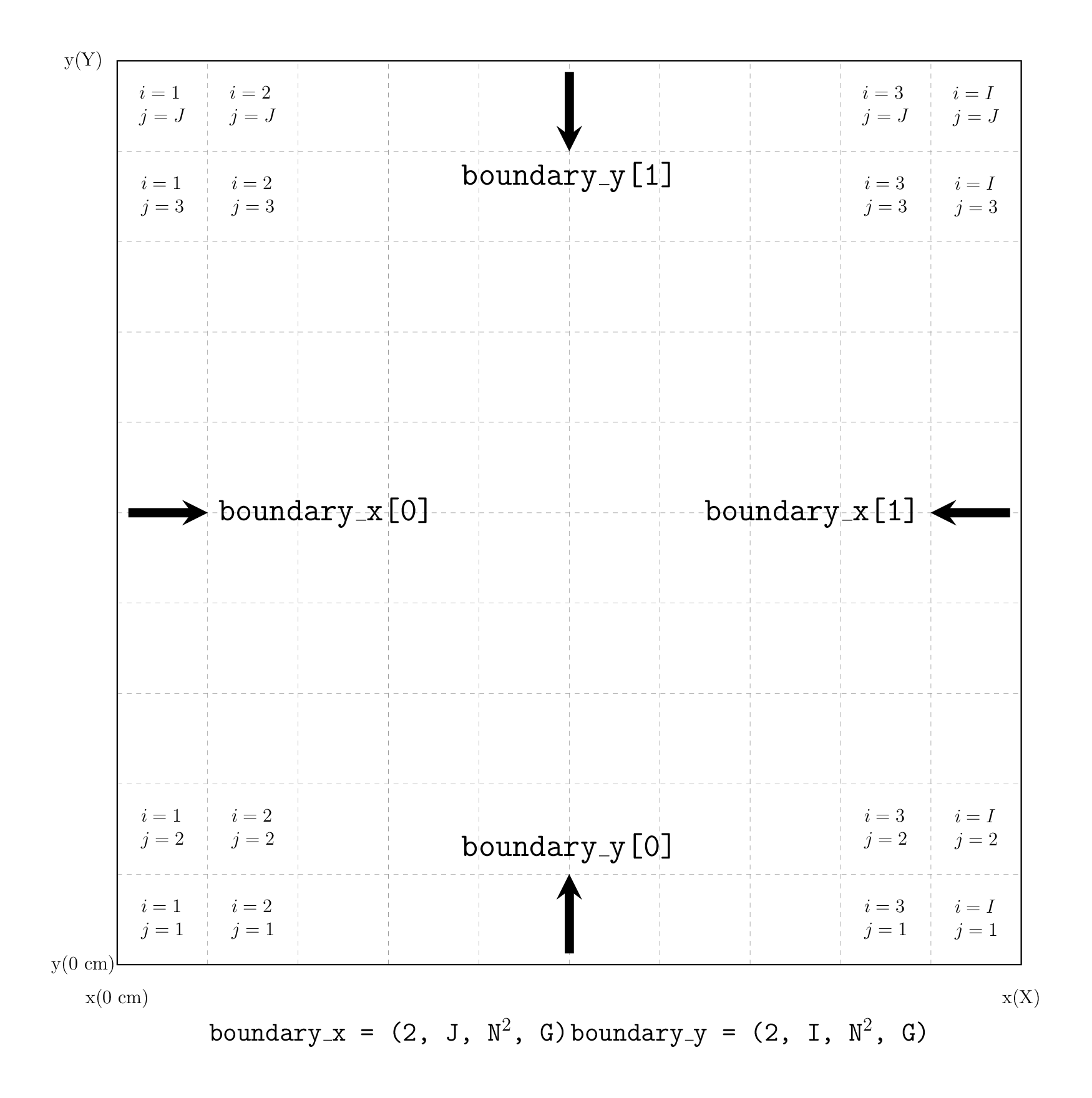
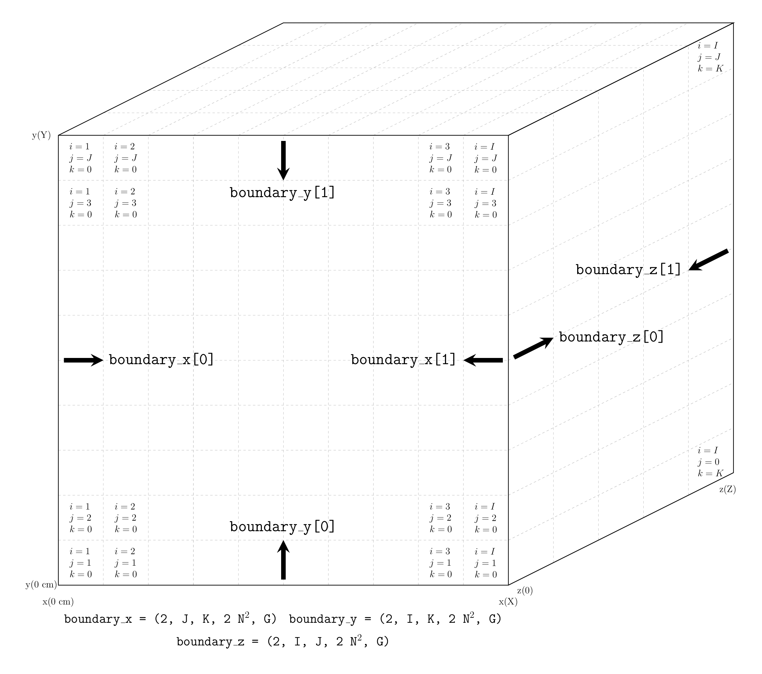
Like the external source, the boundary source terms boundary_x, boundary_y, and
boundary_z (3D) are passed inside the SourceData object. The boundary source requires at least 2 values
for each boundary term (e.g. [x(0), x(X)]). The boundary sources are able to be space-
(for 2D), angle-, energy-, and time-dependent. The minimum broadcasting shapes are shown
in the table below. Figures showing the locations of the boundary sources are also included.
Boundary Source Shapes:
Ndim/Variable |
Problem Type |
Minimum broadcast shape |
Full shape |
|---|---|---|---|
1 / |
Fixed/Critical |
|
|
1 / |
Time-Dependent |
|
|
2 / |
Fixed/Critical |
|
|
2 / |
Time-Dependent |
|
|
2 / |
Fixed/Critical |
|
|
2 / |
Time-Dependent |
|
|
3 / |
Fixed |
|
|
3 / |
Fixed |
|
|
3 / |
Fixed |
|
|
Time-dependent boundary sources only hold the incoming angles. The size of T is
given in Time-Dependent Problems.
The time axis of a time-dependent source rarely needs to be built by hand. ANTS provides helpers that expand a steady source over the time grid:
ants.external1d.time_dependence_constant— repeat a steady external source across all steps (adds the leadingTdimension).ants.boundary1d.time_dependence_constant,ants.boundary1d.time_dependence_decay_01/_02— constant or decaying 1D boundary sources.ants.boundary2d.time_dependence_decay_01/_02/_03— decaying 2D boundary sources.
See Time-Dependent Problems for time-stepping details and the initial-flux shapes.
Compact Sources:
Broadcasting handles a dimension where the source is the same everywhere, but not
one where it is mostly zero. A source in one energy group of an 87-group problem
stores 86 groups of zeros. ants.datatypes.CompactSource stores each distinct
spatial profile once (values, shape (*spatial, S)) and an integer
index of shape (N, G) ((N**2, G) in 2D) giving the profile of each
angle and group, with -1 for a zero source. The spatial shape is (I,) or
(I, J) for external sources and (2,), (2, J), or (2, I) for
boundary sources. Index dimensions of size 1 are broadcast. Any of
external, boundary_x, and boundary_y can be a CompactSource.
from ants.datatypes import CompactSource

# Isotropic source in cells 10-20 of group 0, zero in the other groups
values = np.zeros((cells_x, 1))
values[10:20, 0] = 1.0
index = np.full((1, groups), -1)
index[0, 0] = 0
external = CompactSource(values, index)

# Or from an existing dense array
boundary_x = CompactSource.from_dense(ants.boundary1d.deuterium_tritium(0, edges_g))
The steady-state sweeps read a compact external source through the index, so it is never expanded. Compact boundary sources are expanded to the (surface sized) dense array, and the nearby problems use dense sources.
One-Dimensional Boundary Source

Two-Dimensional Boundary Source
Three-Dimensional Boundary Source
1.2.7. Time-Dependent Initial Flux#
For initial flux shapes (time-dependent problems), see Time-Dependent Problems.