1.7.11.2. Artificial Scattering for Ray Effect Mitigation

Discrete ordinates (S\(_N\)) only transports particles along a finite set of directions. Around a localized source in a weakly scattering medium, the flux streams out along those directions and leaves unphysical streaks between them. These are called ray effects.

ANTS can reduce ray effects with artificial scattering (as-S\(_N\)), following Frank, Kusch, Camminady & Hauck (2020), “Ray Effect Mitigation for the Discrete Ordinates Method Using Artificial Scattering”, Nuclear Science and Engineering. A forward-peaked scattering term is added to the transport equation:

\[\Omega_q \cdot \nabla \psi_q + (\sigma_t + \sigma_{as})\, \psi_q = \sigma_s \phi + \sum_p M_{as}[q, p]\, \psi_p + q_\text{ext}\]

Each row of \(M_{as}\) sums to \(\sigma_{as}\), so the added out-scattering and in-scattering balance and particles are conserved. The kernel only couples nearby ordinates, which smears flux into the gaps between directions.

Artificial scattering is enabled through two SolverData fields:

• sigma_as: the artificial scattering strength (default 0.0, disabled)

• beta_as: the kernel width (default 4.5; larger is wider)

This example solves the same problem three ways:

1. standard S\(_N\) with a coarse quadrature,

2. as-S\(_N\) with the same coarse quadrature, and

3. a fine quadrature as the reference.

import matplotlib.pyplot as plt
import numpy as np
from matplotlib.colors import LogNorm
from scipy.interpolate import RegularGridInterpolator

import ants
from ants.datatypes import (
    GeometryData,
    MaterialData,
    SolverData,
    SourceData,
    SpatialDiscretization,
)
from ants.fixed2d import fixed_source

1.7.11.2.1. Problem setup

A 6 cm x 6 cm pure absorber (\(\sigma_t = 1\) cm\(^{-1}\), no scattering) with a small isotropic source at the center and vacuum boundaries. With no physical scattering to redistribute particles, this is a worst case for ray effects.

Step differencing is used because it keeps the flux positive near the localized source, which is needed for the log-scale plots below.

cells = 100
length = 6.0
delta = np.repeat(length / cells, cells)
centers = (np.arange(cells) + 0.5) * delta[0]

mat_data = MaterialData(
    total=np.array([[1.0]]),
    scatter=np.array([[[0.0]]]),
    fission=np.array([[[0.0]]]),
)

# Isotropic source in the central 4 x 4 cells (0.24 cm x 0.24 cm)
external = np.zeros((cells, cells, 1, 1))
middle = slice(cells // 2 - 2, cells // 2 + 2)
external[middle, middle] = 1.0

sources = SourceData(
    external=external,
    boundary_x=np.zeros((2, 1, 1, 1)),
    boundary_y=np.zeros((2, 1, 1, 1)),
)

geometry = GeometryData(
    medium_map=np.zeros((cells, cells), dtype=np.int32),
    delta_x=delta,
    delta_y=delta,
    bc_x=[0, 0],
    bc_y=[0, 0],
    geometry=3,  # 2D slab
    space_disc=SpatialDiscretization.STEP,
)


def solve(angles, sigma_as=0.0, beta_as=4.5):
    """Return the scalar flux for a quadrature with angles per dimension."""
    quadrature = ants.angular_xy(angles)
    # The lagged artificial scattering source needs more than the default
    # 100 iterations for the larger values of sigma_as below
    solver = SolverData(sigma_as=sigma_as, beta_as=beta_as, max_iter_angular=1000)
    flux = fixed_source(mat_data, sources, geometry, quadrature, solver)
    return flux[..., 0]

1.7.11.2.2. Solving with and without artificial scattering

angular_xy(4) gives 16 directions, which is coarse enough to show strong ray effects. The reference uses angular_xy(32) (1024 directions). At that resolution the flux changes by less than 0.2% from angular_xy(24).

coarse = 4
sigma_as = 7.5

flux_ref = solve(32)
flux_sn = solve(coarse)
flux_as = solve(coarse, sigma_as=sigma_as)


def rel_error(flux):
    return np.linalg.norm(flux - flux_ref) / np.linalg.norm(flux_ref)


print(f"Standard SN relative L2 error: {rel_error(flux_sn):.3f}")
print(f"as-SN       relative L2 error: {rel_error(flux_as):.3f}")

Standard SN relative L2 error: 0.117
as-SN       relative L2 error: 0.082

The flux falls off by several orders of magnitude from the source, so it is plotted on a log scale. All three panels share one color scale.

panels = [
    (flux_sn, f"Standard: angular_xy({coarse})"),
    (flux_as, f"Artificial scattering: angular_xy({coarse}), $\\sigma_{{as}}$ = {sigma_as:g}"),
    (flux_ref, "Reference: angular_xy(32)"),
]
norm = LogNorm(vmin=1e-4, vmax=flux_ref.max())

fig, axes = plt.subplots(1, 3, figsize=(14, 4.6), constrained_layout=True)
for ax, (flux, title) in zip(axes, panels):
    mesh = ax.pcolormesh(
        centers, centers, flux.T, norm=norm, cmap="Blues", shading="auto"
    )
    ax.set_title(title, fontsize=10)
    ax.set_xlabel("x (cm)")
    ax.set_aspect("equal")
axes[0].set_ylabel("y (cm)")
fig.colorbar(mesh, ax=axes, label="Scalar flux", shrink=0.9)
plt.show()

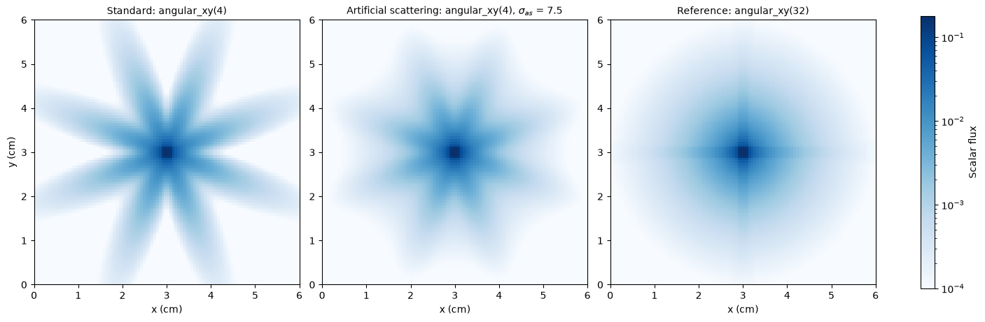
With 16 directions the standard solution is a set of distinct beams with almost no flux between them. Artificial scattering spreads flux into those gaps. The beams are still visible at this strength, but the flux between them is much closer to the reference.

A sharper test is the flux around a circle centered on the source. Without ray effects it should be close to the reference profile at every angle. The reference profile is not perfectly flat because the source is a square on a Cartesian grid.

radius = 2.0
theta = np.linspace(0.0, 0.5 * np.pi, 361)  # one quadrant, by symmetry


def on_circle(flux):
    points = np.column_stack(
        [0.5 * length + radius * np.cos(theta), 0.5 * length + radius * np.sin(theta)]
    )
    return RegularGridInterpolator((centers, centers), flux)(points)


fig, ax = plt.subplots(figsize=(8, 4.2))
ax.plot(np.degrees(theta), on_circle(flux_ref), color="#52514e", lw=2,
        ls="--", label="Reference: angular_xy(32)")
ax.plot(np.degrees(theta), on_circle(flux_sn), color="#2a78d6", lw=2,
        label=f"Standard: angular_xy({coarse})")
ax.plot(np.degrees(theta), on_circle(flux_as), color="#eb6834", lw=2,
        label=f"Artificial scattering: $\\sigma_{{as}}$ = {sigma_as:g}")
ax.set_xlabel("Angle around source (degrees)")
ax.set_ylabel(f"Scalar flux at r = {radius:g} cm")
ax.set_xlim(0, 90)
ax.set_xticks(np.arange(0, 91, 15))
ax.grid(alpha=0.3)
ax.spines[["top", "right"]].set_visible(False)
ax.legend(frameon=False, loc="upper center", bbox_to_anchor=(0.5, -0.16), ncol=3)
plt.show()

ratio_sn = on_circle(flux_sn).mean() / on_circle(flux_ref).mean()
ratio_as = on_circle(flux_as).mean() / on_circle(flux_ref).mean()
total_as = flux_as.sum() / flux_ref.sum()
print(f"Mean flux on the circle / reference: standard {ratio_sn:.2f}, as-SN {ratio_as:.2f}")
print(f"Total flux / reference:              as-SN {total_as:.3f}")

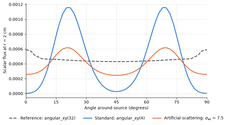
Mean flux on the circle / reference: standard 0.99, as-SN 0.86
Total flux / reference:              as-SN 1.010

Artificial scattering reduces the oscillation, but it also lowers the flux on the circle relative to the reference. This is a bias of the method in an absorber. Each artificial scattering event redirects a particle slightly, so the particle travels a longer path to reach the circle, and more particles are absorbed on the way. The total flux, which is proportional to total track length, is slightly higher than the reference for the same reason.

1.7.11.2.3. Choosing \(\sigma_{as}\)

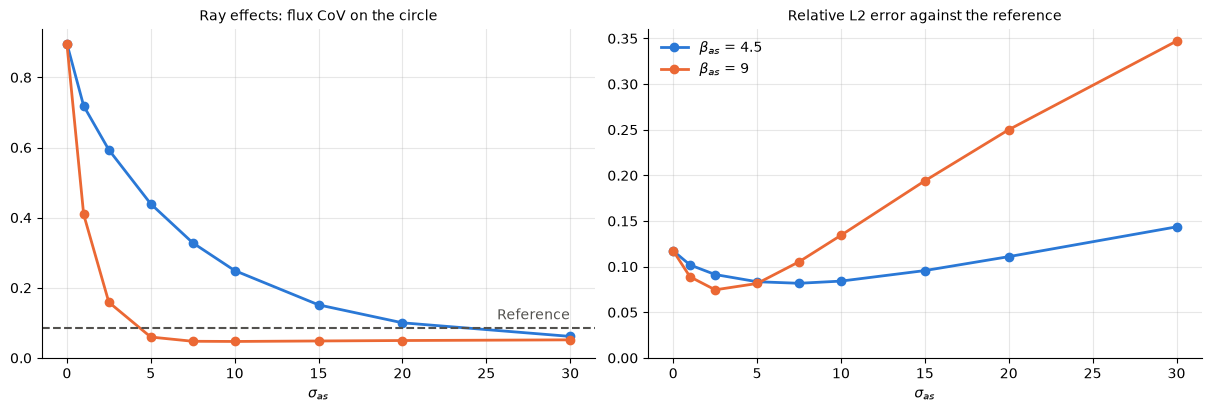
Artificial scattering trades ray effects for added smoothing. Too little leaves the beams in place. Too much over-smooths the solution and acts like a real scattering medium. The sweep below tracks two measures:

• the coefficient of variation (CoV) of the flux on the circle above, which measures how strong the ray effects are, and

• the relative L2 error against the reference over the whole domain.

The sweep is run for the default kernel width, beta_as = 4.5, and for a kernel twice as wide, beta_as = 9. Larger sigma_as also needs more source iterations, because the artificial in-scattering term is lagged between iterations. This is why solve raises max_iter_angular, and ANTS warns if the iterations stop at the limit before converging.

sweep = np.array([0.0, 1.0, 2.5, 5.0, 7.5, 10.0, 15.0, 20.0, 30.0])
widths = {4.5: "#2a78d6", 9.0: "#eb6834"}
cov, error = {}, {}
for beta_as in widths:
    cov[beta_as], error[beta_as] = [], []
    for value in sweep:
        flux = solve(coarse, sigma_as=value, beta_as=beta_as)
        ring = on_circle(flux)
        cov[beta_as].append(ring.std() / ring.mean())
        error[beta_as].append(rel_error(flux))

ring_ref = on_circle(flux_ref)
cov_ref = ring_ref.std() / ring_ref.mean()

fig, (ax0, ax1) = plt.subplots(1, 2, figsize=(12, 4), constrained_layout=True)
for beta_as, color in widths.items():
    label = f"$\\beta_{{as}}$ = {beta_as:g}"
    ax0.plot(sweep, cov[beta_as], color=color, lw=2, marker="o", ms=6, label=label)
    ax1.plot(sweep, error[beta_as], color=color, lw=2, marker="o", ms=6, label=label)
ax0.axhline(cov_ref, color="#52514e", lw=1.5, ls="--")
ax0.annotate("Reference", (sweep[-1], cov_ref), xytext=(0, 6),
             textcoords="offset points", ha="right", color="#52514e")
ax0.set_title("Ray effects: flux CoV on the circle", fontsize=10)
ax0.set_ylim(bottom=0)

ax1.set_title("Relative L2 error against the reference", fontsize=10)
ax1.set_ylim(bottom=0)
ax1.legend(frameon=False)

for ax in (ax0, ax1):
    ax.set_xlabel("$\\sigma_{as}$")
    ax.grid(alpha=0.3)
    ax.spines[["top", "right"]].set_visible(False)
plt.show()

for beta_as in widths:
    print(f"beta_as = {beta_as:g}")
    for value, c, e in zip(sweep, cov[beta_as], error[beta_as]):
        print(f"  sigma_as = {value:5.1f}   CoV = {c:.3f}   L2 error = {e:.3f}")

beta_as = 4.5
  sigma_as =   0.0   CoV = 0.896   L2 error = 0.117
  sigma_as =   1.0   CoV = 0.719   L2 error = 0.102
  sigma_as =   2.5   CoV = 0.593   L2 error = 0.091
  sigma_as =   5.0   CoV = 0.439   L2 error = 0.083
  sigma_as =   7.5   CoV = 0.328   L2 error = 0.082
  sigma_as =  10.0   CoV = 0.249   L2 error = 0.084
  sigma_as =  15.0   CoV = 0.151   L2 error = 0.096
  sigma_as =  20.0   CoV = 0.100   L2 error = 0.111
  sigma_as =  30.0   CoV = 0.061   L2 error = 0.144
beta_as = 9
  sigma_as =   0.0   CoV = 0.896   L2 error = 0.117
  sigma_as =   1.0   CoV = 0.409   L2 error = 0.089
  sigma_as =   2.5   CoV = 0.159   L2 error = 0.075
  sigma_as =   5.0   CoV = 0.060   L2 error = 0.082
  sigma_as =   7.5   CoV = 0.048   L2 error = 0.105
  sigma_as =  10.0   CoV = 0.047   L2 error = 0.134
  sigma_as =  15.0   CoV = 0.048   L2 error = 0.194
  sigma_as =  20.0   CoV = 0.050   L2 error = 0.250
  sigma_as =  30.0   CoV = 0.052   L2 error = 0.347

With the default kernel width, the overall error is lowest around \(\sigma_{as} \approx 5\)-\(10\) for this problem, but the ray effects fall slowly. The CoV only reaches the reference value near \(\sigma_{as} \approx 25\), where the flux on the circle is far too low. The wider kernel moves flux further with each artificial scattering event, so it removes the ray effects with less \(\sigma_{as}\) and less bias, and it gives the lowest error, around \(\sigma_{as} \approx 2.5\). Past the best value the extra smoothing costs more accuracy than it recovers. Once the CoV drops below the reference value, the solution is smoother than the true flux, which is a clear sign of too much artificial scattering. The best values depend on the problem, the quadrature and the mesh, so it is worth running a short sweep like this one for new problems.

1.7.11.2.4. Notes

• Artificial scattering is available in the 2D solvers: fixed2d, timed2d (all time discretizations) and hybrid2d, and in the 3D fixed3d. It has no effect when sigma_as = 0. It is not used by critical2d or vhybrid2d.

• beta_as sets the kernel width \(\epsilon = \beta / N_q\), where \(N_q\) is the number of directions on the full sphere, as in Frank et al. (2020). angular_xy(N) keeps the \(N^2\) directions in the upper hemisphere, so \(N_q = 2 N^2\). Each 2D direction also receives the artificial scattering of its reflection through the x-y plane, so a 2D problem has the same artificial scattering as a 3D problem that does not change in z. Frank et al. use about 4.5 for explicit and 4.0 for implicit schemes, but a coarse quadrature like the one here can do better with a wider kernel.

• Artificial scattering does not replace angular refinement. It makes a coarse quadrature more usable, but the converged answer still comes from a finer quadrature.