

1.3. Homogenized Zones with Multiple Materials#
In this analysis, the two-dimensional space for the deterministic neutron transport equation is represented as a series of quadrilaterals. A triangular mesh has been shown to be effective [LM93], but it would alter the discretization schemes presented in the spatial discretization section. While this does not present an issue with media that use quadrilateral shaped materials, it severely limits the types of two-dimensional problems that can be simulated. To allow for additional material shapes in two-dimensional spaces, namely cylinders and triangles, a homogenization process is used for each spatial cell.
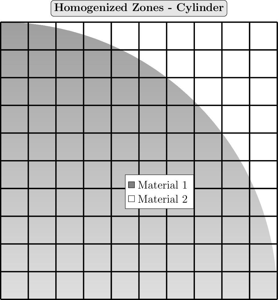
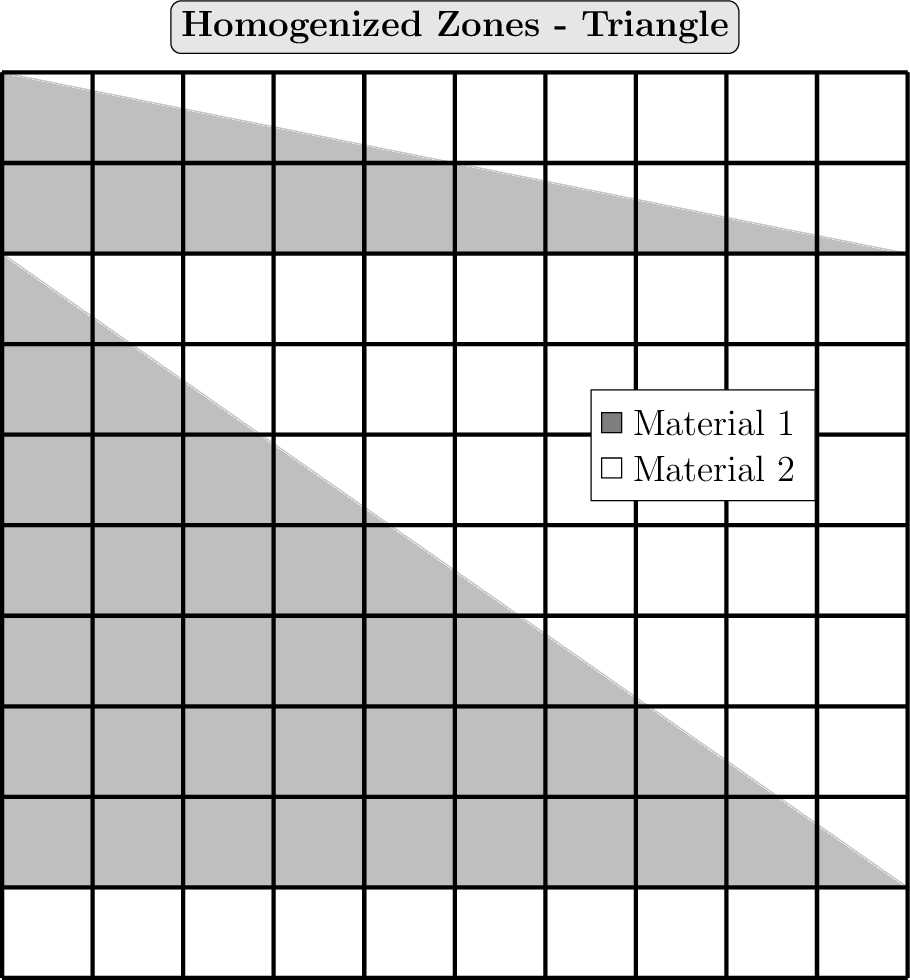
In this regime, either a cylinder or triangle is overlaid on the Cartesian grid, as shown in the figures below. For each spatial cell which contains regions of both materials, a composite material is created using
where \(\sig[1]{t}\) and \(\sig[2]{t}\) are the original materials and
\(\rho\) is the percentage of the first material present in the cell. This
allows for preservation of the cross-sectional information of the spatial cell
without requiring the exact shape. To prevent having an excessive number of
materials through this homogenization process, the \(\rho\) values can be
rounded with the decimals argument (four decimal places is usually enough).
Homogenized Zones — Cylinder
Homogenized Zones — Triangle
A Monte Carlo approach was taken to determine the \(\rho\) values for the cylindrical shape. A quarter cylinder, as seen in the cylinder figure, is used and propagated over the four quadrants for the full cylinder. A uniform distribution is sampled across the medium in both the \(x\) and \(y\) directions where the specific spatial cell is determined \((i, j)\) for each particle \((x_{n}, y_{n})\). The sample radius \(r_{n}\) is calculated for each particle which determined the material the sample point is occupying. This is added to the tally of the corresponding material for each spatial cell which can be normalized to calculate the \(\rho\) values. A quarter cylinder was used for symmetry across each quadrant and a sufficient number of samples were used for an accurate approximation of the zone homogenization.
The \(\rho\) values for the triangle shape were calculated using finite elements. The general structure of the triangle used with the Cartesian grid is shown in the triangle figure, where the vertices of the triangle are represented as \((x_{1}, y_{1})\), \((x_{2}, y_{2})\), and \((x_{3}, y_{3})\). As with the cylinder shape, a uniform distribution is sampled across the medium to calculate the spatial cell \((i, j)\) for the particle. To determine the material each particle is currently in, a function can be created using the triangle shape functions from finite elements [LdO10]. The global coordinates of the triangle vertices can be transformed onto the local coordinate system represented as \((\xi, \eta)\). The three shape functions are calculated as \(\xi\), \(\eta\), and \(1 - \xi - \eta\) in which the function to determine the correct medium is
in which \(f(\xi, \eta) \geq 0\) is inside or on the edge of the triangle and \(f(\xi, \eta) < 0\) is outside the triangle. The transformation is carried out as
where \((x_{1}, y_{1})\), \((x_{2}, y_{2})\), and \((x_{3}, y_{3})\) are the vertices of the triangle and \((x_{n}, y_{n})\) is the sample point. A sufficient number of samples and normalization is used to determine the material percentages \(\rho\).
The weight matrix is then converted to a medium map, with one new material for
each unique set of \(\rho\) values. The same is done for three-dimensional
weight matrices of shape (cells_x, cells_y, cells_z, materials).
- ants.weight_spatial2d(weight_matrix, xs_total, xs_scatter, xs_fission, chi=None, decimals=None)[source]#
Convert a 2D weight matrix to a medium map and mixed cross sections.
Each unique set of material weights becomes a new material, where the cross sections are the volume weighted sums of the original materials.
- Parameters:
weight_matrix (ndarray of float, shape (cells_x, cells_y, materials)) – Fraction of each material in each spatial cell.
xs_total (ndarray, shape (materials, groups)) – Total cross sections.
xs_scatter (ndarray, shape (materials, groups, groups[, L + 1])) – Scatter cross sections, with or without Legendre moments.
xs_fission (ndarray, shape (materials, groups, groups)) – Fission cross sections, or shape
(materials, groups)whenchiis given.chi (ndarray, shape (materials, groups), optional) – Fission spectrum. It is weighted by the neutrons produced in each material (
xs_fissionsummed over groups), which is exact when only one material in the mixture is fissile.decimals (int, optional) – Round the weights to this many decimal places before finding the unique mixtures. This limits the number of new materials.
- Returns:
medium_map (ndarray of int32, shape (cells_x, cells_y)) – Index of the mixed material in each spatial cell.
xs_total (ndarray, shape (materials, groups)*) – Mixed total cross sections.
xs_scatter (ndarray, shape (materials, groups, groups[, L + 1])*) – Mixed scatter cross sections.
xs_fission (ndarray) – Mixed fission cross sections, with the same trailing shape as the input.
chi (ndarray, shape (materials, groups)*) – Mixed fission spectrum, only returned when
chiis given.
- ants.weight_spatial3d(weight_matrix, xs_total, xs_scatter, xs_fission, chi=None, decimals=None)[source]#
Convert a 3D weight matrix to a medium map and mixed cross sections.
Same as
weight_spatial2d(), butweight_matrixhas shape(cells_x, cells_y, cells_z, materials)and the returnedmedium_maphas shape(cells_x, cells_y, cells_z).
1.4. Preset Two-Dimensional Layouts#
The homogenization above is applied in practice by
ants.main.weight_matrix2d (Monte Carlo zone fractions for curved/triangular
shapes) and ants.main.spatial2d (exact integer maps for rectangular regions).
The ants.utils.mesh2d module bundles these into ready-made benchmark
layouts. Each helper returns either a weight matrix of shape
(cells_x, cells_y, materials) (homogenized fractions per cell) or an integer
medium map of shape (cells_x, cells_y) — both consumable as the
medium_map input described in Standard Inputs.
Layout |
Output |
Description |
|---|---|---|
|
weight matrix |
Single fissile cylinder embedded in void. |
|
weight matrix |
Fuel core + reflector annulus embedded in void. |
|
weight matrix |
Four triangular fuel regions in an HDPE moderator (9 × 9 cm benchmark). |
|
medium map |
2D C5G7 MOX fuel assembly benchmark (7 materials, rectangular regions). |
1.4.1. Layout factory functions#
- ants.utils.mesh2d.cylinder_1mat(cells_x, cells_y, length_x=None, length_y=None, radius=None, N_particles=None)[source]#
Weight matrix for a single fissile cylinder embedded in void.
- Parameters:
cells_x (int) – Number of spatial cells in x.
cells_y (int) – Number of spatial cells in y.
length_x (float, optional) – Domain length in x [cm]. Default is
2 * radius.length_y (float, optional) – Domain length in y [cm]. Default is
2 * radius.radius (float, optional) – Cylinder radius [cm]. Default is 4.279960.
N_particles (int, optional) – Monte Carlo samples. Default is
cells_x * 50_000.
- Returns:
weight_matrix – Material weight fractions. Material 0 = fuel cylinder, material 1 = void background.
- Return type:
ndarray of float, shape (cells_x, cells_y, 2)
- ants.utils.mesh2d.cylinder_2mat(cells_x, cells_y, length_x=None, length_y=None, r_inner=None, r_outer=None, N_particles=None)[source]#
Weight matrix for a fuel core + reflector annulus embedded in void.
- Parameters:
cells_x (int) – Number of spatial cells in x.
cells_y (int) – Number of spatial cells in y.
length_x (float, optional) – Domain length in x [cm]. Default is
2 * r_outer.length_y (float, optional) – Domain length in y [cm]. Default is
2 * r_outer.r_inner (float, optional) – Inner (fuel) cylinder radius [cm]. Default is 3.0.
r_outer (float, optional) – Outer (reflector) annulus radius [cm]. Default is 4.5.
N_particles (int, optional) – Monte Carlo samples. Default is
cells_x * 50_000.
- Returns:
weight_matrix – Material weight fractions. Material 0 = inner fuel, 1 = reflector annulus, 2 = void background.
- Return type:
ndarray of float, shape (cells_x, cells_y, 3)
- ants.utils.mesh2d.double_chevron(cells_x, cells_y, N_particles=None)[source]#
Weight matrix for the 9 x 9 cm double-chevron benchmark geometry.
Four triangular uranium fuel regions in an HDPE moderator background, matching the geometry encoded in examples/weight_matrix_2d_chevron.npy.
- Parameters:
cells_x (int) – Number of spatial cells in x.
cells_y (int) – Number of spatial cells in y.
N_particles (int, optional) – Monte Carlo samples. Default is
cells_x * cells_y * 40.
- Returns:
weight_matrix – Material weight fractions. Material 0 = uranium fuel, material 1 = HDPE background.
- Return type:
ndarray of float, shape (cells_x, cells_y, 2)
- ants.utils.mesh2d.c5g7(cells_x=153, cells_y=153)[source]#
Medium map for the 2D C5G7 MOX fuel assembly benchmark.
Based on M.A. Smith et al. NEA/NSC/DOC(2003)16, Appendix A. Returns an integer medium map (not a weight matrix) because the C5G7 geometry consists entirely of rectangular regions with no curved boundaries.
- Parameters:
cells_x (int, optional) – Number of spatial cells in x. Default is 153 (= 51 * 3).
cells_y (int, optional) – Number of spatial cells in y. Default is 153 (= 51 * 3).
- Returns:
medium_map – Material index per cell. 0=moderator, 1=UO2, 2=MOX43, 3=MOX70, 4=MOX87, 5=guide tube, 6=fission chamber.
- Return type:
ndarray of int, shape (cells_x, cells_y)
- Raises:
ValueError – If cells do not align with the 1.26 cm pin pitch.
- ants.utils.mesh2d.resize_weight_matrix(weight_matrix, new_cells_x, new_cells_y)[source]#
Expand or shrink a weight matrix (or medium map) to a new grid size.
- Parameters:
weight_matrix (ndarray) – Float array of shape (cells_x, cells_y, materials), or integer array of shape (cells_x, cells_y).
new_cells_x (int) – Target number of cells in x.
new_cells_y (int) – Target number of cells in y.
- Returns:
resized – Array with shape (new_cells_x, new_cells_y, materials) for float inputs, or (new_cells_x, new_cells_y) for integer medium maps. Float outputs are renormalized so weights sum to 1 along axis 2.
- Return type:
ndarray
1.4.2. Command-line interface#
The same layouts can be generated (and optionally plotted or saved) from the command line:
# Generate a layout
python -m ants.utils.mesh2d <layout> --cells-x N --cells-y N [--plot] [--save out.npy]

# Example: a 100 x 100 single-cylinder weight matrix, saved to disk
python -m ants.utils.mesh2d cylinder-1mat --cells-x 100 --cells-y 100 --save cyl.npy

# Resize an existing weight matrix or medium map to a new grid
python -m ants.utils.mesh2d --resize cyl.npy --cells-x 200 --cells-y 200 --save cyl200.npy
Layout-specific overrides (e.g. --radius, --r-inner / --r-outer,
--length-x / --length-y, --n-particles) are available for the Monte
Carlo cylinder layouts.